
Here is a set of basic Excel formulas, grouped by task. The examples use English function names and commas as argument separators. Excel in another language may use different function names or separators—for example, Russian Excel commonly uses semicolons—while the calculation logic stays the same.
For examples tied specifically to a renovation estimate, see the 101 article How to calculate in Excel? (in Russian). It shows the basic pattern: quantity × price, copying the formula down, and adding a total row.
Contents:
How can you read Excel formulas and avoid mistakes?
A formula may look straightforward in one cell. Once you copy it down, surprises appear: a range moves, a header reference is lost, or a price comes from the wrong row. Two habits help.
First, decide which references should move when you copy the formula and which should stay fixed. The dollar sign locks a reference: $A$1 fixes both column and row; $A1 fixes the column; A$1 fixes the row.
Second, keep numeric values as numbers. If a price is accidentally stored as text, some formulas may return errors or zeros. In the default cell format, numbers usually align to the right and text to the left; this is a quick clue to check.
Arithmetic and cell references
These formulas form the starting point for most estimates and accounting tables.
Take an estimate row with quantity in B2, price in C2 and amount in D2.
- =B2*C2 — multiplication, giving the line amount.
- =B2+C2, =B2-C2 and =B2/C2 — addition, subtraction and division.
- =ROUND(D2,0) — rounding to whole rubles in the original example. For kopecks, or two decimal places: =ROUND(D2,2).
- =ABS(D2) — the absolute value, useful if negative values appear.
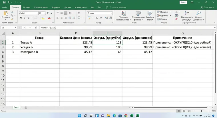
The screenshot comes from the Russian example; use the English function names in the formulas above. Round deliberately: rounding each line can give a different total from rounding the overall sum. Estimates commonly keep line amounts to two decimal places and round the final total.
Sums, averages, minimums and maximums
These functions answer “how much altogether?” and “what is the typical price?” In an estimate, the result may be a section or project total. In an expense table, it may cover a week, month or project.
- =SUM(D2:D200) — total of a range.
- =AVERAGE(C2:C200) — average price.
- =MIN(C2:C200) and =MAX(C2:C200) — lowest and highest values.
- =COUNT(D2:D200) — number of cells containing numbers.
- =COUNTA(D2:D200) — number of nonempty cells, including text and formulas that return an empty string.
If a long table has blank rows, allow some room in the range and calculate from a column that is consistently filled in, such as “Amount.”
How do you count and sum by criteria?
Once you classify rows by section, work type, project, contractor or expense category, a simple sum is not enough. You may need to “count materials only,” “sum project no. 3 only,” or “find spending on tiling work.”
- =SUMIF(A:A,"Materials",D:D) — sum by one criterion.
- =COUNTIF(A:A,"Work") — count rows matching a condition.
- =AVERAGEIF(A:A,"Delivery",C:C) — average values matching a condition.
For several criteria, use the corresponding functions with an “S” suffix.
- =SUMIFS(D:D,A:A,"Materials",C:C,">0") — sum materials with a positive price.
- =COUNTIFS(A:A,"Materials",C:C,">0") — count material rows with a positive price.
A similar approach to expense tracking appears in the 101 article How to track expenses in Excel? (in Russian): with many expenses, figures lose meaning unless you group them by category and apply conditions.
Logic and errors
Logic functions automate rules often stated in words: “apply a discount if there is one,” “do not calculate an amount until quantity and price are entered,” or “show a blank instead of a division-by-zero error.”
- =IF(OR(B2="",C2=""),"",B2*C2) — calculate the amount only when both quantity and price are present.
- =AND(A2<>"",C2>0) — test two conditions together.
- =OR(A2="Materials",A2="Work") — accept either category.
- =IFERROR(B2/C2,"") — return an empty string if division produces an error.
Division often appears when an estimate calculates a percentage discount or margin. If the denominator is zero, Excel returns an error. IFERROR can save the time spent cleaning up those expected errors by hand.
Lookups and reference tables
A reference table is a sheet that holds the source values: a price list, work items, norms or coefficients. The calculation sheet keeps an item code or name and retrieves the price automatically. This reduces manual entry and helps keep prices consistent across projects. In the examples below, E2 holds the item code. For VLOOKUP and MATCH, codes are in the first column of the “Price List” sheet; for HLOOKUP, they are in its first row.
- =VLOOKUP(E2,'Price List'!A:D,4,FALSE) — find a value in the first column of the reference table and return the value from column four.
- =HLOOKUP(E2,'Price List'!A1:Z3,3,FALSE) — the horizontal version for a reference table arranged in rows.
- =INDEX('Price List'!D:D,MATCH(E2,'Price List'!A:A,0)) — a flexible INDEX and MATCH combination that can replace VLOOKUP.
Modern Excel versions also provide XLOOKUP. It searches a lookup range and returns a matching value from a return range without a column number. If XLOOKUP is unavailable, INDEX with MATCH remains a widely compatible alternative.
If your price lists and estimates already live in Excel, you do not have to retype them when moving to the 101 App. See Fast estimate import from Excel into the 101 App (in Russian).
Text, dates and dynamic arrays
Text formulas help when imported data is messy: extra spaces, joined names, item codes or comments. Dates are useful for expense periods, work deadlines and planned-versus-actual reporting.
- =LEN(A2) — length of the text.
- =LEFT(A2,5), =RIGHT(A2,5) and =MID(A2,3,4) — extract part of a string.
- =TRIM(A2) — remove extra spaces.
- =TEXT(DATE(2026,2,3),"dd.mm.yyyy") — turn a date into formatted text, useful for exports.
- =TODAY() and =NOW() — the current date and the current date and time.
- =DATE(G2,H2,I2) — build a date using the year in G2, month in H2 and day in I2.
If your Excel version supports dynamic arrays, you can build lists that update with the source data. You can filter, sort and extract unique values without a pivot table.
- =FILTER(A2:D200,A2:A200="Materials","") — return matching rows.
- =SORT(A2:D200,4,-1) — sort by the fourth column in descending order.
- =UNIQUE(A2:A200) — list unique values.
How do you build a small estimate template with formulas?
This short sequence gives you a working estimate in Excel. You can extend it with sections, discounts, markups, actual expenses and payments.
- Create columns for Section, Item, Unit, Quantity, Price, Amount and Comment.
- In the Amount column, enter the multiplication formula =D2*E2 and copy it down.
- Add a table total: =SUM(F2:F200).
- Add a section total with SUMIF: =SUMIF(A:A,"Rough-in",F:F).
- If you have a price list, retrieve prices with VLOOKUP or INDEX and MATCH.
- Handle a price lookup error: =IFERROR(VLOOKUP(B2,'Price List'!A:D,4,FALSE),"").
As the number of workbooks grows, it becomes harder to identify the latest version, manage access and protect formula integrity. We discuss these issues in Excel or the 101 App for estimates and financial tracking? (in Russian) and continue in Excel or the 101 App for project tracking (in Russian).
If you want to show a client a clear estimate without assembling reports by hand, see how online estimate calculation works (in Russian) and how to build an estimate from scratch in the 101 App (in Russian).